Physical and computational background of the line profile calculation#
In the following documentation, we will discuss the origin of molecular and atomic lines and what they look like. After that, we will explain how the line profiles are calculated in line racer.
Line shapes and broadening mechanisms#
This section is about the line profile and atomic and molecular state transitions. The content is mostly based on Demtröder, 2016 (a classic German physics textbook). A more complete and detailed explanation in english can be found in Chapter 2 of David’s Master’s thesis, which can be found here. Throughout this text, we will use wavenumbers \(\nu\) in units of \(\mathrm{cm}^{-1}\) as our spectral coordinate, which is common in spectroscopy. Molecular and atomic spectral lines arise from transitions between different energy levels of atoms or molecules. The energy level can be associated with electronic states of atoms and molecules, and vibrational or rotational states of molecules. Also combinations thereof are possible. When an atom or molecule transitions from a higher energy level to a lower one, it emits a photon with an energy equal to the difference between the two levels. Conversely, when it absorbs a photon with the right energy, it can transition from a lower energy level to a higher one. Even though these transitions occur at specific energies (or wavenumbers/wavelengths), the observed spectral lines are not infinitely sharp (so not described by a delta function). Instead, they have a certain width and shape, which is described by the line profile or line shape function. There are three mechanisms that contribute to the broadening of spectral lines: natural broadening, pressure (collisional) broadening, and thermal broadening.
Natural and collisional broadening#
Natural and collisional broadening are both described by a Lorentzian profile. Natural broadening arises from the inherent uncertainty in the energy levels of atoms and molecules due to the finite lifetime of excited states, as described by the Heisenberg uncertainty principle. From a semi-classical perspective this can be modeled as a damped oscillator, which has a spectral power density that follows a Lorentzian profile with a width determined by the lifetime of the state. Collisional broadening, also known as pressure broadening, occurs when atoms or molecules collide with each other. These collisions can excite or de-excite a molecule or atom into a different state. The associated effect on state lifetimes leads to a broadening of the spectral lines, likewise due to the Heisenberg uncertainty principle, also in the shape of a Lorentzian. The Lorentzian profile is given by:
where \(\nu\) is the wavenumber, \(\nu_0\) is the line center, \(\delta_\text{p}\) is the pressure shift coefficient, \(P\) is the pressure and \(\gamma\) is the broadening parameter of the line. The broadening parameter \(\gamma\) can be parameterized as:
where \(\gamma_\text{nat}\) is the natural broadening parameter and \(\gamma_\text{col}\) is the collisional broadening parameter, \(\tau = 1/A_{ij}\) is the lifetime of the excited state with \(A_{ij}\) being the Einstein coefficient, \(p_b\) is the partial pressure of the broadening species \(b\), \(\gamma_b\) is the collisional broadening coefficient for the broadening species \(b\) at a reference temperature \(T_\text{ref}\) and \(n_b\) is the temperature exponent for the broadening species \(b\). The different broadening parameters can be added, since the broadening mechanisms are independent of each other (the convolution of two Lorentzian with widths \(\gamma_a\) and \(\gamma_b\) is again a Lorentzian with width \(\gamma = \gamma_a + \gamma_b\)). We note that broadening is line-dependent, that is, \(A_{ij}\), \(\gamma_b\), \(n_b\), etc., change from line to line.
For molecules, the line and perturber specific broadening parameters \(\gamma_b\) and \(n_b\) are provided directly in the line list (for HITRAN/HITEMP) or are calculated from the provided broadening parameters for the different vibrational and rotational states (for ExoMol). For atoms, the broadening parameters are usually calculated based on potential of the van-der-Waals interaction between the atom and the perturber. The potential is given by \(V(r) = -\frac{C_6}{r^6}\), where \(C_6\) is the van-der-Waals coefficient and \(r\) is the distance between the atom and the perturber. The broadening parameters are then calculated based on the van-der-Waals coefficient and the temperature, as described in Mihalas (1978):
where \(v\) is the relative velocity of the atom and the perturber and \(n_\text{pert}\) density of the perturbing species. The \(C_6\) is calculated based on Unsöld (1955) as:
where \(e\) is the elementary charge, \(\alpha\) is the polarizability of the perturber and \(\overline{r^2}\) is the mean square radius of the valence electron of the atom, which can be calculated as:
with \(a_0\) being the Bohr radius, \(n^*\) being the effective principal quantum number of the state and \(l\) being the orbital quantum number of the state and \(Z_\text{eff}\) being the effective nuclear charge. The effective principal quantum number is an estimation of the principal quantum number of the state and is given by:
with \(R_H\) being the Rydberg constant, \(E_\text{ion}\) being the ionization energy of the atom and \(E_\text{state}\) being the energy of the state.
The line shift is calculated as \(\Delta\nu\)
Thermal broadening#
Thermal broadening, also known as Doppler broadening, arises from the thermal motion of atoms and molecules and the associated Doppler effect. Due to their motion, the emitted or absorbed photons from an ensemble of atoms and molecules have a broader energy distribution than just being a delta function at the res-frame transition wavenumber, which directly translates into a broader line profile. The thermal broadening is described by a Gaussian profile given by:
where \(\nu\) is the wavenumber, \(\nu_0\) is the line center and \(\gamma_D\) is the Doppler width given by:
where \(\nu_0\) is the line center, \(k_\text{B}\) is the Boltzmann constant, \(T\) is the temperature, \(m\) is the mass of the atom or molecule and \(c\) is the speed of light. Compared to the usual definition of the standard deviation \(\sigma_D\) of a Gaussian distribution, the introduced definition \(\gamma_D\) relates as \(\gamma_D = \sqrt{2}\sigma_D\).
Voigt profile#
Since the broadening mechanisms are independent of each other, the overall line profile is given by the convolution of the individual profiles. Intuitively, this can be understood from the fact that at any given wavenumber those atoms and molecules can absorb light whose Lorentz broadened line profiles have been Doppler shifted enough to have a non-negligible cross-section at the wavenumber in question. The resulting profile is known as the Voigt profile, which can be seen in the following figure as the dashed line.
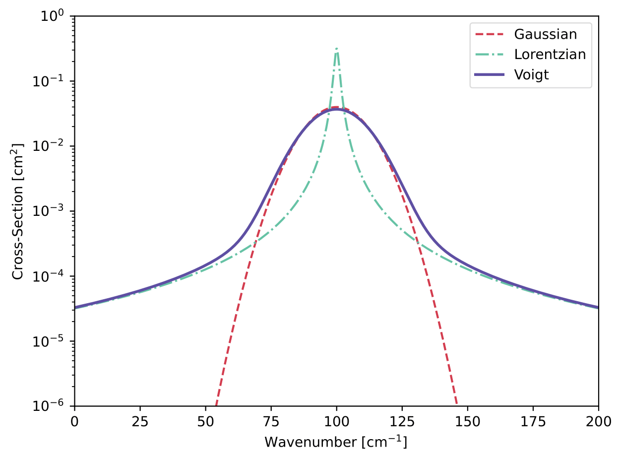
We note here that the Voigt profile is only an approximation of the real line profile, since other effects are neglected here. However, the Voigt profile is widely used in astrophysics and atmospheric physics due to its simplicity and good accuracy for many applications, which is why it is also used in line racer. Nevertheless, other line profiles exist, such as the Hartmann-Tran Profile (HTP).
Cutoff and sub-Lorentzian treatment of the line wings#
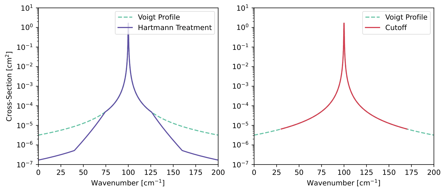
Describing pressure broadening through a Lorentz profile makes simplifying assumptions that start to break down especially far away from the line core (e.g., the orientation of the approaching collisions partners can matter, as well as the detailed physical modeling of the collision). Line racer provides two different options to account for this, by treating the far wings of the Voigt profile in a special way. The first one is a simple cutoff of the wings, since it is unphysical for the wings to extend infinitely far. However, it is an ongoing debate in the community about where to set the cutoff. There are studies like Gharib-Nezhad et al. 2023 which suggest that the cutoff should be set between 25 \(\mathrm{cm}^{-1}\) and 100 \(\mathrm{cm}^{-1}\) from the line center. The general impact of a cutoff is illustrated in the right panel of the following figure.
The second option is a sub-Lorentzian treatment of the wings, which reduces the absorption in the far wings compared to the Voigt profile. This is done by multiplying the Lorentzian part of the Voigt profile with a factor that decreases with distance from the line center. We implement several sub-Lorentzian treatments. The Hartmann et al. 2002 sub-Lorentzian treatment, which was originally measured for CH4 lines that were collisionally broadened by H2. However, it is also used as an approximation for other molecules and broadening species in the absence of better data and therefore is our standard recommendation for all molecules. Specifically for CO2, we also provide the sub-Lorentzian treatment from Burch et al. 1969 The general impact of the sub-Lorentzian treatment is illustrated in the left panel of the following figure.
In general, we suggest to use a cutoff no larger than 100 \(\mathrm{cm}^{-1}\), if no sub-Lorentzian treatment is used. If a sub-Lorentzian treatment is used, a larger cutoff can be chosen, or even neglected, since the far wings are already reduced by the sub-Lorentzian treatment. However, we suggest to still use a cutoff of 100 \(\mathrm{cm}^{-1}\), also for computational speed. Additionally, we usually use the sub-Lorentzian treatment, since it is more physical than a simple cutoff. If you have a different opinion about the cutoff or sub-Lorentzian treatment or if you recommend implementing a different sub-Lorentzian treatment, please feel free to contact us; we are happy to discuss this important topic.
Line calculation in line racer#
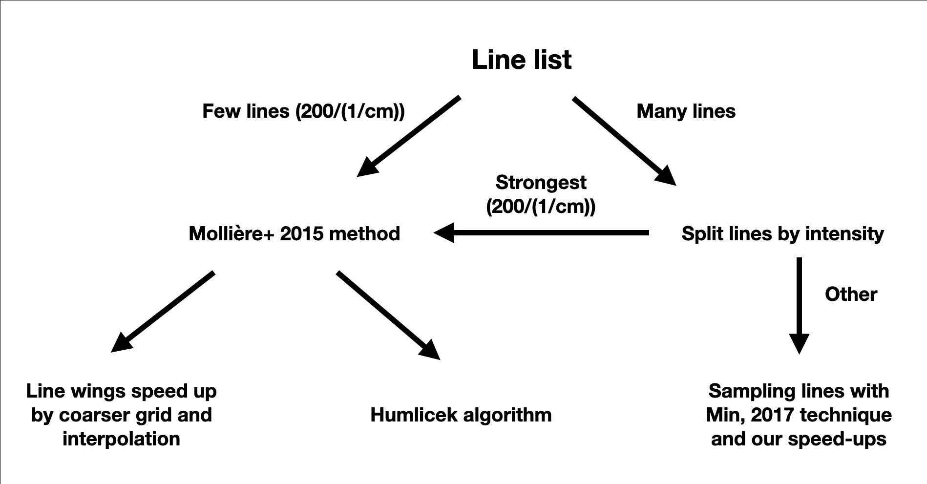
Since the Voigt profile is a convolution, it is computationally expensive to calculate, especially if the line lists contain billions of lines. Therefore, the line profile calculation in line racer is split into two different methods depending on the size of the line list. If the line list is sparse, which is here defined as less than 200 lines per 1 \(\mathrm{cm}^{-1}\), the Mollière et al. 2015 method is used. If the line list contains more lines, for every 1 \(\mathrm{cm}^{-1}\) interval, the 200 strongest lines are calculated with the Mollière et al. 2015 method. The remaining “weak” lines are calculated using a sampling technique of the line profile, which was proposed by M. Min 2017, and further improved by us. It is also shown graphically in the following figure.
Mollière et al. 2015 method#
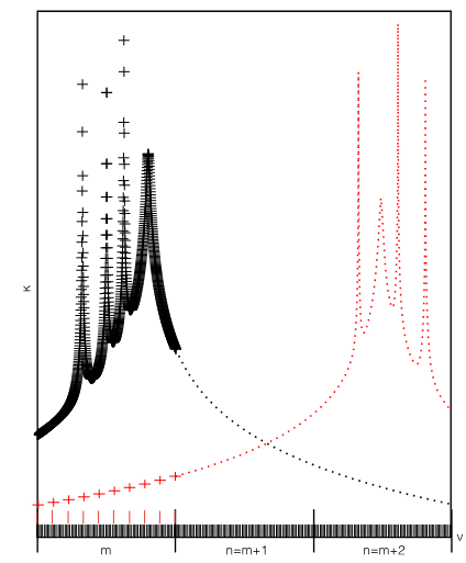
The first method is adapted from Mollière et al. 2015 and uses the Humlícek, 1982 algorithm to calculate the line profiles. However, since the Humlícek algorithm is computationally expensive, Mollière et al. 2015 introduced a speedup for the far wings of the lines. It calculates the line cores on the full resolution of the grid and uses a coarser grid for the wings of the lines and then interpolates it back to the full grid. The whole grid is divided into sub grids. More specifically, if a subgrid \(n \neq m\) is located far away from sub grid \(m\), the line profile is only calculated on the coarse grid of \(m\) and then interpolated back to the full grid. This speedup is illustrated in the following figure, which is taken from Mollière et al. 2015. The black crosses indicate the calculation of the line profile on the full resolution in sub grid \(m\), while the red crosses indicate the calculation on the coarse grid and then interpolated back to the full grid. A further explanation can be found in the paper, including the criteria when to switch to the coarse grid calculation.
Sampling technique#
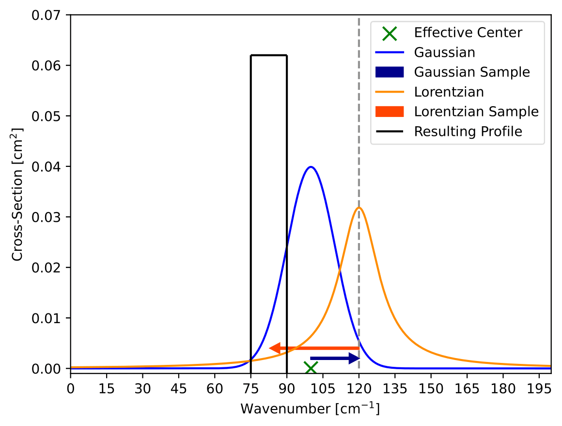
The sampling technique is based on M. Min 2017. This elegant method has the advantage that the lines profiles are not calculated on every wavenumber grid point, but are rather sampled randomly according to the desired precision. This means that lines that are very weak and only contributing to the background can be handled with a low number of samples and therefore at a higher speed. On the other hand, strong lines can be sampled with a large number of samples and therefore a higher precision. This leads to a significant speedup in the line profile calculation, especially for large line lists with many weak lines. To sample the lines, a Gaussian and a Lorentzian shift away from the line core position are drawn and added. These represent the thermal and collisional/natural broadening, respectively. Adding two random numbers drawn from different distributions is equivalent to drawing a random number from the convolution of the two distributions, which is the Voigt profile in our case. Therefore, to obtain the Voigt profile, the sum of the samples is added to the center location of the line \(\nu_0\) and in the wavenumber bin, that contains the sampled value, a weight is added. In the simplest case, one can just add 1 and normalize the profile afterward. However, you could also directly use 1/N, with N being the number of samples, to obtain a normalized profile directly, assuming bin widths of 1. An illustration of this procedure is shown in the following figure. The green cross represents the line center, while the blue function is a Gaussian profile and the orange function is a Lorentzian profile. The orange arrow indicates a drawn Lorentzian sample, while the blue arrow indicates a drawn Gaussian sample. To better visualize the convolution, the dashed grey line shows that the Lorentzian sample is shifted by the drawn Gaussian sample. In the bin that contains the sampled Voigt value, a weight is added, as indicated by the black histogram box. This would be a line sampled with one sample, assuming bin widths of 15 \(\mathrm{cm}^{-1}\).
However, taking only one sample per line is not sufficient to obtain a good approximation of the Voigt profile for more important lines. Nevertheless, the background opacity can be constrained with that very well. To sample lines more accurately, more samples must be drawn. With more and more samples, the profile converges to the real Voigt profile. An illustration of that is shown in the following gif, where the number of samples is increasing from 1 to 1 000 000.
This approach to approximating a convolution is interesting, but it takes a lot of samples to describe a Voigt profile accurately, especially on high resolution grids. Therefore, M. Min 2017 proposed a speedup technique, the derivation of which is described in detail in his paper, and reproduced in David’s thesis. It basically makes more use of one sample by not just adding the weight in the bin that contains the sampled value, but spreads out a weight \(w\) in an interval defined from the line center plus the Gaussian \(\Delta\nu_\mathrm{therm}\) and then plus and minus the Lorentzian sample \(\Delta\nu_\mathrm{press}\). By that, more information is obtained from one sample and therefore less samples are needed to obtain a good approximation of the Voigt profile. The following gif shows the increasing number of samples for the improved sampling technique compared to the slow one shown before. It can be shown analytically that this approach converges to a Voigt profile for appropriately chosen weights \(w\), the expression for which was derived in M. Min 2017.
To achieve even higher speeds, we further improved this method. For the speed up technique M. Min 2017 proposed, the profiles have to be normalized after the sampling. We introduced a new expression for the weights \(w\), which ensures that sampled lines are already normalized and speeds up the calculation even more. The significant difference to the previous method is that instead of adding \(w = \frac{\Delta\nu_\mathrm{press}^2}{\Delta\nu_\mathrm{press}^2 + \gamma^2}\) to all bins in the sampled interval, we are adding the following:
where \(N_\mathrm{samples}\) is the number of samples, \(\Delta\nu_\mathrm{press}\) is the pressure broadening scaled Lorentzian sample, \(\gamma\) is the Lorentzian width, \(S\) is the line strength, \(\nu_\mathrm{eff}\) is the effective wavenumber of the line and \(R\) is the resolution of the grid. The first part accounts for spreading the weight according to the Lorentzian sample, the second part normalizes the profile according to the number of samples and the line strength, while the last part accounts for the grid bin width. For a logarithmic grid, it has the stated shape. More details about the derivation, further explanations and detailed comparisons can be found in the master’s thesis of David, which can be found here.
Moreover, to get the best possible performance, we also adapted a method from de Regt et al. 2025, which uses a grid resolution that adapts to the width of the lines. By that, no information is lost, but also no unnecessary high resolution is used for broad lines. This is used for the grid on which the lines are sampled. Results are then interpolated back to the original grid.