Using HITRAN line lists#
A guide on how to download HITRAN line lists can be found in the downloading line list data tutorial. To download HITRAN data, you need to be logged in on the HITRAN website. Therefore, we will download the demonstration data from a cloud, just to show how the calculation works. If you want to use the HITRAN data for real, please download the line list files from the HITRAN website.
We will calculate the HITRAN CO2 line list here. Credit for the data goes to these papers. First we need to import the relevant packages and set up the folder structure.
[1]:
import numpy as np
import matplotlib.pyplot as plt
import line_racer.line_racer as lr
import urllib.request
import zarr.storage
import os

# if you want to use the conversion to the pRT format
import petitRADTRANS

lr.LineRacer.check_installation()

os.makedirs('line_list/CO2', exist_ok=True)
Running line racer installation test...
line racer installation test passed successfully.
After that, we are downloading the line list data. As mentioned, it is downloaded from a cloud using urllib.request. If that is not working for you, please download it manually from HITRAN or here. However, the partition function can be downloaded from the HITRAN website directly. For HITRAN data the .par file is needed, which contains all line information, especially the broadening for air and self. If you want to use more
or other broadening species, please have a look at the downloading line list data tutorial. Additionally, the partition function data is needed, which is stored in a .txt file.
[2]:
urllib.request.urlretrieve('https://keeper.mpdl.mpg.de/f/3b4ddd913b7e44e984fe/?dl=1', 'line_list/CO2/69300f3e.par')
urllib.request.urlretrieve("https://hitran.org/data/Q/q7.txt", "line_list/CO2/q7.txt")
[2]:
('line_list/CO2/q7.txt', <http.client.HTTPMessage at 0x175e6b8d0>)
As for ExoMol, we need to define the pressure and temperature grid. Here, we are only using one pressure and temperature point for demonstration purposes. If you want to use a pre-defined petitRADTRANS grid, you can use the function lr.LineRacer.prt_pressure_temperature_grid() as shown in the ExoMol example.
[3]:
pressures = [1.0]  # in bar
temperatures = [1500.0]  # in K
After that, we can define the line racer object, which already contains most of the relevant information for our opacity calculation. In general, everything is written in lower case letters, except for the line list name, since it is only used for naming the output files.
[4]:
CO2_racer = lr.LineRacer(resolution=1e6,
                         cutoff=100.0,  # in 1/cm
                         lambda_min=1.1e-5,  # in cm
                         lambda_max=2.5e-2,  # in cm
                         grid_type='log',
                         sublorentzian="Burch",  # Attention, ONLY for CO2! Hartmann is default, but since we are calculating CO2 here, we use the Burch et al. 1969 sub-Lorentzian treatment
                         database='hitran',
                         input_folder='line_list/CO2/',  # path to folder with input files
                         temperatures=temperatures,  # in K
                         pressures=pressures,  # in bar
                         species_isotope_dict={'12C-16O2': 1.0},  # dictionary with the name of the isotope(s) in ExoMol convention and their number fraction(s)
                         line_list_name='HITRAN2024',
                         broadening_species_dict={'air': 1.0},
                         broadening_type='hitran_table',  # could also be 'sharp_burrows', 'hitran_table' or 'constant'

                         # Change the following only if you know what you do!
                         force_molliere2015_below_wn=40,  # use the Mollière et al. 2015 method for lines with effective wavenumbers smaller than this threshold
                         force_molliere2015_below_pressure=0.01,  # in bar. Only use the force_molliere2015_method_below_wn for pressures below this pressure
                         force_molliere2015_method=False  # whether to force using Mollière et al. (2015) for line profile calculation, recommended only if warning appears or for small line lists
                         )
A detailed description of the class constructor can be found in the ExoMol section. Here, we will just explain the differences.
The input folder where the line list files (.par/.out, .txt) are stored is now the one containing the HITRAN files, the naming convention of the dictionary with the isotopes to calculate is still in the ExoMol naming convention and will be translated internally. Since the HITRAN line lists do not have specific names, we just call it ‘HITRAN2024’. For the dictionary with the broadening species air and self are possible for .par files, since their information is included there.
For self-created .out files the species names as seen on the HITRAN website in the output format description are required as an input here. As a broadening type, the ‘hitran_table’ is used, which stands for the broadening parameters included in the .par or .out file. The molecular mass is not required for HITRAN line lists, since it is read from the molparam.txt file automatically.
An important note here is, that for the sub-Lorentzian treatment, the default is the Hartmann et al. (2002) method. However, since we are calculating CO2 opacities here, it is recommended to use the Burch et al. (1969) method (ONLY for CO2!), which is specifically designed for CO2 and gives better results. Therefore, we set sublorentzian="Burch" here. If you want to use the Hartmann et al. (2002) method, you can just set sublorentzian="Hartmann".
The explanation for force_molliere2015_method, force_molliere2015_below_wn and force_molliere2015_below_pressurecan be found in the ExoMol section.
HITRAN intensities are weighted by their natural abundance by default. In line racer, this is automatically corrected for and the opacities are scaled to abundance 1. If you want a different abundance, such as the natural abundance, you can set the desired abundance in the species_isotope_dict.
We also need to prepare the calculation by setting up the wavelength grid. Finally, we can provide the transition files list directly here, or let line racer search for all .par or .out files in the input folder. If there are .par and .out files, the .out files are preferred.
[5]:
transition_files_list = CO2_racer.prepare_opacity_calculation()
print("The transition file(s) to be used for the calculation are: ", transition_files_list)
The transition file(s) to be used for the calculation are: ['line_list/CO2/69300f3e.par']
After preparing the calculation, we can start the actual opacity calculation. Here, we can also choose whether to use MPI for parallelization or not. If you are on a cluster and have MPI set up, you can set use_mpi=True to use it. Otherwise, just set it to False and line racer will use multiprocessing for parallelization. In the case of normal multiprocessing (use_mpi=False) you can choose the number of cores by setting n_cores to
the number of cores you want to use.
If you are using the line_racer_obj.calculate_opacity in a script make sure to put it in a if __name__ == "__main__": block to avoid problems with multiprocessing.
You can either directly use the petitRADTRANS format by setting prt_format=True or first calculate the cross-sections in line racer’s own format, which is a zarr compressed with zip. More about that, and which further information are needed for the petitRADTRANS format can be found in the ExoMol section. Here, they are set to None. We use the flag verbose=True, to get more information about the line calculation.
For calculations with HITRAN line lists additionally to the intensity correction files, the molparam.txt file is needed, which is downloaded automatically if not present in the data/ folder. More about the intensity correction can be found in the ExoMol section and the intensity correction chapter.
[6]:
final_cross_section_file_name = CO2_racer.calculate_opacity(transition_files_list,
                                                            use_mpi=False,
                                                            n_cores=1,
                                                            sampling_boost=1.0,
                                                            coarse_grid_switch=True,

                                                            # pRT output options
                                                            prt_format=False,
                                                            doi=None,
                                                            additional_information=None,
                                                            use_prt_input_file_path=False,

                                                            # more output
                                                            verbose=True)

print("The cross-sections are stored in the file: ", final_cross_section_file_name)
Using cutoff and Burch intensity correction grid and interpolated to 100.0 1/cm
Reading HITRAN transition file...
Finished reading HITRAN transition file in 1.17 seconds.


 Line parameter calculation time: 0.014775753021240234 s
Starting the line profile calculation of 174446 lines

 Starting internal lines!
Line profile calculation done
 Internal lines done!
 Starting external lines!
Progress: 770/773 subgrids
 External lines done!
Total time for opacity calculation:  48.963690996170044 s

The cross-sections are stored in the file:  cross-sections/cross-section_12C-16O2__HITRAN2024__40-90909cm-1.zarr.zip
The resulting cross-section file is stored in the folder cross-sections/ by default. The file contains the pressure grid in bar and temperature grid in Kelvin, the wavenumber grid in 1/cm and the cross-sections in \(\rm cm^2/molecule\) for each pressure and temperature point. If you want to convert the cross-sections to the petitRADTRANS format, you could directly set prt_format=True in the calculate_opacity function or just convert it afterward, as explained in the ExoMol
section.
[7]:
store = zarr.storage.ZipStore(final_cross_section_file_name, mode='a')
z = zarr.group(store=store)

# Access datasets
pressures = z['pressures'][:]
temperatures = z['temperatures'][:]
wavenumbers = z['wavenumbers'][:]
cross_section = z['cross-sections']

print("Pressures (bar): ", pressures)
print("Temperatures (K): ", temperatures)

# Extract slice and plot
cross_section_slice = cross_section[:]
Pressures (bar):  [1.]
Temperatures (K):  [1500.]
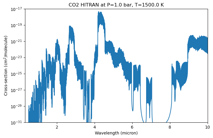
[8]:
fig, ax = plt.subplots(figsize=(8, 5))
ax.plot(1/wavenumbers * 1e4, cross_section_slice[0, 0, :])  # convert wavenumber to wavelength in micron

ax.set_xlabel('Wavelength (micron)')
ax.set_ylabel('Cross-section (cm$^2$/molecule)')
ax.set_title(f'CO2 HITRAN at P={pressures[0]} bar, T={temperatures[0]} K')
ax.set_yscale('log')
ax.set_ylim(1e-31, 1e-17)
ax.set_xlim(0.3, 10);