Using ExoAtom line lists

To start with the opacity calculation we need to load the relevant packages and check if line racer is installed correctly.

import numpy as np
import matplotlib.pyplot as plt
import line_racer.line_racer as lr
import urllib.request
import zarr.storage
import os

# if you want to use the conversion to the pRT format
import petitRADTRANS

lr.LineRacer.check_installation()

Running line racer installation test...
line racer installation test passed successfully.

We need to download all the required files, which is also explained in the downloading line list data tutorial. Here, we will download the Li line list NIST as an example. First of all, we are creating the folder structure.

os.makedirs('line_list/Li', exist_ok=True)

After that, we are downloading the line list data. For ExoAtom, always the .states file is needed and the .trans files of the required wavelength region. Additionally, the .pf partition function file is required as well.

base = "https://www.exomol.com/exoatom/db/Li/NIST"
files = {
  f"{base}/Li__NIST.states" : "line_list/Li/Li__NIST.states",
  f"{base}/Li__NIST.trans" : "line_list/Li/Li__NIST.trans",
  f"{base}/Li__NIST.pf" : "line_list/Li/Li__NIST.pf",
}
for url, dest in files.items():
  if not os.path.exists(dest):
      urllib.request.urlretrieve(url, dest)

The last step before setting up the calculation is to choose the pressure and temperature grid. If you want to calculate your opacities for usage in petitRADTRANS, you can use their standard grid. It is stored in line racer. However, you can also define your own grid. The following command shows you how to use the pRT grid, but after that we are only using one pressure and temperature for demonstration purposes.

pressures, temperatures = lr.LineRacer.prt_pressure_temperature_grid()
print("petitRADTRANS pressure grid (in bar): ", pressures)
print("petitRADTRANS temperature grid (in K): ", temperatures)

pressures_demo = [1e-3]  # in bar
temperatures_demo = [1500.0]  # in K

petitRADTRANS pressure grid (in bar):  [1.0e-06 1.0e-05 1.0e-04 1.0e-03 1.0e-02 1.0e-01 3.2e-01 1.0e+00 3.2e+00
 1.0e+01 3.2e+01 1.0e+02 3.2e+02 1.0e+03]
petitRADTRANS temperature grid (in K):  [  81.  109.  148.  200.  270.  365.  493.  575.  666.  770.  899. 1050.
 1215. 1400. 1614. 1800. 2000. 2217. 2500. 2750. 2995. 3250. 3500. 3750.
 4000.]

After that, we can define the line racer object, which already contains most of the relevant information for our opacity calculation. In general, everything is written in lower case letters, except for the line list name, since it is only used for naming the output files.

Li_racer = lr.LineRacer(resolution=1e6,  # lambda / Delta lambda = 1,000,000
                        cutoff=1000.0,  # in 1/cm, Attention: default is 100 1/cm
                        lambda_min=1.1e-5,  # in cm
                        lambda_max=2.5e-2,  # in cm
                        grid_type='log',  # So lambda / Delta lambda is constant at all lambda
                        database='exoatom',
                        sublorentzian=None,  # currently no sub-Lorentzian treatment available for atoms, so set to None
                        input_folder='line_list/Li/',  # path to folder with input files
                        temperatures=temperatures_demo,  # in K
                        pressures=pressures_demo,  # in bar
                        mass=6.941, # in amu, not a list, since exoatom line lists contain only one isotope per file
                        species_isotope_dict={'Li-NatAbund': 1.0},  # dictionary with the name of the isotope(s) in ExoMol convention and their number fraction(s)
                        line_list_name='NIST',
                        broadening_species_dict={'H2': 0.85, 'He': 0.15},
                        broadening_type='van der waals',  # only option for ExoAtom so far

                        # Change the following only if you know what you do!
                        force_molliere2015_below_wn=40,  # use the Mollière et al. 2015 method for lines with effective wavenumbers smaller than this threshold.
                        force_molliere2015_method=False  # whether to force using Mollière et al. (2015) for line profile calculation, recommended only if warning appears or for small line lists. The whole line list will be calculated with this method
                         )

The parameters we defined here are the following: The resolution of the wavelength grid we want to calculate the opacities on in the format of \(\lambda/\Delta\lambda\), the cutoff of the line wings (default is 100/cm), the sub-Lorentzian treatment (currently none available for atoms), the minimum and maximum wavelength in cm (here the full pRT grid), the grid type (currently just logarithmic possible, which means a constant \(\lambda/\Delta\lambda\) for all lambda), the database we want to use (here ExoAtom), the input folder where the line list files (.states, .trans, .pf) are stored, the temperature grid in Kelvin, the pressure grid in bar, the molecular mass in amu (can be found in the .adef.json file on ExoAtoms’s website), a dictionary with isotopes we want to consider in the ExoMol naming convention and their abundances (for the atoms in ExoAtom mainly -NatAbund, since all isotopes are included), the line list name (here NIST), a dictionary with the broadening species and their abundances and finally the broadening type. For atoms, there is currently just the van der Waals broadening available, which is calculated with the Unsöld (1955) approximation. Additionally, a line shift is also applied, which is calculated with the same approximation. More about the line broadening and line shift can be found in the background information of the line calculation.

Since the calculation of the line broadening is dependent on the ionization energy of the atom, which is already included into the code, it is important, that the isotope name is correctly specified, so that the correct ionization energy is used. For almost all isotopes in ExoAtom, the name is the element name followed by ‘-NatAbund’, since all isotopes are included. For example, for carbon it would be ‘C-NatAbund’. If you want to calculate the opacity for a specific isotope, you can specify that as well, but make sure to use the correct name as given on the ExoAtom website. For example, for the isotope 2H (Deuterium) it would be ‘2H’. Additionally, if you want to calculate the opacity of an ion, you need to specify that in the isotope name as well, for example for C+ it would be ‘C-NatAbund_p’. If you have any problems with the naming, please check the ExoAtom website or contact us.

Additionally, there is one parameter: force_molliere2015_method, which forces the usage of the Mollière et al. (2015) method for line profile calculation. This is only recommended for small line lists or if you get warnings that the default method fails. It increases the calculation time significantly for large line lists. More about this method can be found in the background information of the line calculation. Related, there is force_molliere2015_below_wn (default 40). If set to a wavenumber in 1/cm, all lines with effective wavenumber below this threshold are calculated with the Mollière et al. (2015) method, while the rest of the line list uses the default mix between the two methods. This is useful when calculating opacities far into the infrared: once the cutoff becomes comparable to the line position itself, the sampling method becomes very slow when only the line wing is contributing. The Mollière et al. (2015) treatment stays reasonable fast, which is why you can force it to be used for these lines. This is only relevant when calculating opacities at wavenumbers smaller than 100/cm (larger than 100µm). A good choice for the variable is therefore the grid boundary of the grid, so for the standard grid 40/cm (250µm). Unlike force_molliere2015_method, this only switches the affected lines, so the runtime cost is even improved.

After defining the racer object, we can start the opacity calculation. The first step is to prepare the opacity calculation. Here, the wavelength grid is set up and the transition files list is either created by the function, or you can directly input it. If you do not provide it, line racer will search for all transition files (with .trans extension, if none found for .trans.bz2 extension) in the input folder.

transition_files_list = Li_racer.prepare_opacity_calculation()  # or Li_racer.prepare_opacity_calculation(transition_files_list=[list, of, the, files])

print("The transition file(s) to be used for the calculation are: ", transition_files_list)

The transition file(s) to be used for the calculation are:  ['line_list/Li/Li__NIST.trans']

After preparing the calculation, we can start the actual opacity calculation with the calculate_opacity() method. Here, we can also choose whether to use MPI for parallelization or not. If you are on a slurm cluster and have MPI set up, you can set use_mpi=True to use it. If you have done so, you do not need to specify the number of cores, but just follow the instructions in the tutorial on how to use line racer on a cluster. If you are not using a slurm cluster or do not have MPI set up, just set use_mpi=False and line racer will use multiprocessing for parallelization. In this case of normal multiprocessing (use_mpi=False) you have to choose the number of cores by setting n_cores to the number of cores you want to use.

If you are using the line_racer_obj.calculate_opacity in a script make sure to put it in a if __name__ == "__main__": block to avoid problems with multiprocessing.

The opacity can directly be output in the petitRADTRANS format by setting prt_format=True. However, we will explain that later. Here, we are first calculating the cross-sections in line racer’s own format, which is a zarr compressed with zip. To directly save it in the petitRADTRANS format, just use the same parameters we will explain below. Here, they are set to None.

Additionally, we are using the flag verbose=True, to get more information about the line calculation. This should be set to False if you want to run the calculation with maximum speed. The most important information is already printed without verbose mode.

If you want to assure that all output is correctly written to the terminal, run the script with python -u script.py or run export PYTHONUNBUFFERED=1 before the script.

As a first step of the calculation, the intensity corrections of the lines to take the cutoff into account are prepared. If you do that for the first time, line racer will download the files needed. More about that in the chapter to intensity correction.

final_cross_section_file_name = Li_racer.calculate_opacity(transition_files_list,
                                                            use_mpi=False,
                                                            n_cores=1,
                                                            sampling_boost=1.0,
                                                            coarse_grid_switch=True,

                                                            # pRT output options
                                                            prt_format=False,
                                                            doi=None,
                                                            additional_information=None,
                                                            use_prt_input_file_path=False,

                                                            # more output
                                                            verbose=True)

print("The cross-sections are stored in the file: ", final_cross_section_file_name)

Using cutoff intensity correction grid and interpolated to 1000.0 1/cm
Reading ExoAtom states file...
Reading ExoAtom states file...
Finished reading ExoAtom states file in 0.00 seconds.

Finished reading ExoAtom states file in 0.00 seconds.
Reading ExoAtom transition file...
Finished reading ExoAtom transition file in 0.00 seconds.

 Line parameter calculation time: 0.0013349056243896484 s
Starting the line profile calculation of 257 lines

 Starting internal lines!
Line profile calculation done Internal lines done!
 Starting external lines!
Progress: 770/773 subgrids
 External lines done!

Total time for opacity calculation:  5.1801416873931885 s

The cross-sections are stored in the file:  cross-sections/cross-section_Li-NatAbund__NIST__40-90909cm-1.zarr.zip

Please note that most of the time is spent in downloading the intensity correction files. If you have already downloaded them once, the calculation will be much faster.

The resulting cross-section file is stored in the folder cross-sections/ by default. The file contains the pressure grid in bar and temperature grid in Kelvin, the wavenumber grid in 1/cm and the cross-sections in \(\rm cm^2/molecule\) for each pressure and temperature point. If you want to convert the cross-sections to the petitRADTRANS format, you could directly set prt_format=True in the calculate_opacity function.

The other additional options for the upper function are the sampling_boost, which can be used to increase the number of samples used to sample the weak lines. This increases the accuracy of the opacity calculation, but also the calculation time. The number of samples per line is already set to a good value by default, so changing this is usually not necessary. The last parameter is coarse_grid_switch, which controls whether to use an adaptive grid, which fits to the average width of the lines, so that only a required number of wavelength points are used to resolve the lines. This usually speeds up the calculation significantly. It is strongly recommended to keep it on, since there is no information lost. This feature was adapted from de Regt et al. 2025.

After calculating the opacities, we can plot them. Since we only used one pressure temperature point, we will just plot that one here. The line racer internal file format is a zarr compressed with zip, which can be read in easily with the zarr package.

# Open read-only ZipStore
store = zarr.storage.ZipStore(final_cross_section_file_name, mode='a')
z = zarr.group(store=store)

# Access datasets
pressures = z['pressures'][:]
temperatures = z['temperatures'][:]
wavenumbers = z['wavenumbers'][:]
cross_section = z['cross-sections']

print("Pressures (Bar): ", pressures)
print("Temperatures (K): ", temperatures)

# Extract slice and plot
cross_section_slice = cross_section[:]

Pressures (Bar):  [0.001]
Temperatures (K):  [1500.]

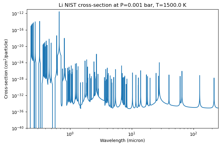
The cross-sections are stored in a 3D array with the shape (n_pressures, n_temperatures, n_wavenumbers). Here, we only have one pressure and temperature point, so we can just extract the first slice of the array. After that, we can plot the cross-sections.

fig, ax = plt.subplots(figsize=(8, 5))
ax.plot(1/wavenumbers * 1e4, cross_section_slice[0, 0, :])  # convert wavenumber to wavelength in micron
ax.set_xlabel('Wavelength (micron)')
ax.set_ylabel('Cross-section (cm$^2$/particle)')
ax.set_title(f'Li NIST cross-section at P={pressures[0]} bar, T={temperatures[0]} K')
ax.set_yscale('log')
ax.set_xscale('log')
ax.set_xlim(0.2, 250)
ax.set_ylim(1e-40, 1e-11);

If you want to convert the file to the pRT format afterward, you can use the following function. For that you need to have a working petitRADTRANS installation. A guide on how to install petitRADTRANS can be found here.

If you use the pRT format, please provide the DOI of the line list you used for the calculation, so that it is stored in the file. Additionally, you can provide information you want to include into the file. The standard information includes the isotope list, the line racer version, the line list name, the broadening species dictionary, the broadening type, the cutoff and whether Hartmann corrections were used.

The rewrite parameter controls whether to overwrite an already existing file with the same name. If you want to keep the old file if one exists, set it to False. Additionally, if you want to use the petitRADTRANS input file path for storing the converted file, set use_prt_input_file_path=True. Note, that if you choose that and rewrite=True, your current pRT opacities are overwritten. If set to False, the files are stored in the prt format, but in a folder in the current working directory called cross-sections_prt_format/. It will automatically calculate the opacities in the standard correlated-k and line-by-line format of petitRADTRANS.

add_info = "this was a test calculation of Li opacities using line racer."
doi = "10.18434/T4W30F"  # doi of the line list

Li_racer.convert_opacity_to_prt_format(final_cross_section_file_name, doi, rewrite=True, additional_information=add_info, use_prt_input_file_path=False)

Generating petitRADTRANS wavenumber grid... Done.
Reading opacity files in directory '.temporary_pRT_xsec_Li-NatAbund_NIST'...
Starting conversion of directory '.temporary_pRT_xsec_Li-NatAbund_NIST'...
 Reading file '.temporary_pRT_xsec_Li-NatAbund_NIST/xsec_Li-NatAbund_1.00e-03bar_1500K.zarr' (1/1)... Done.
Preparation successful
Starting line-by-line conversion (boundaries: [ 0.3 28. ])...
 Writing line-by-line file '/Users/haegele/codes/line_racer/docs/content/notebooks/cross-sections_prt_format/opacities/lines/line_by_line/Li/Li-NatAbund/Li__NIST.R1e6_0.3-28mu.xsec.petitRADTRANS.h5'...
Successfully converted files in '.temporary_pRT_xsec_Li-NatAbund_NIST' to line-by-line pRT files
Starting correlated-k conversion (R = 1000)...
 Reshaping...
 Initializing correlated-k parameters...
 Calculating correlated-k (13/7728)...

/Users/haegele/codes/line_racer/.pixi/envs/default/lib/python3.11/site-packages/petitRADTRANS/__file_conversion.py:3139: UserWarning: directory '.temporary_pRT_xsec_Li-NatAbund_NIST' contains only 1 files, the standard petitRADTRANS temperature-pressure grid size is 130; a finer temperature-pressure grid allows for a more accurate interpolation of the cross-sections
  warnings.warn(f"directory '{opacities_directory}' contains only {len(opacity_files)} files, "

 Done.lating correlated-k (7728/7728)...
 Writing file '/Users/haegele/codes/line_racer/docs/content/notebooks/cross-sections_prt_format/opacities/lines/correlated_k/Li/Li-NatAbund/Li__NIST.R1000_0.1-250mu.ktable.petitRADTRANS.h5'...
Successfully converted files in '.temporary_pRT_xsec_Li-NatAbund_NIST' to correlated-k pRT files
Removed temporary folder .temporary_pRT_xsec_Li-NatAbund_NIST with the individual p T point files.

We can ignore the warning about the number of files, since we only used one pressure temperature point for demonstration purposes. In practice, you would use the whole line list or at least all files covering the wavelength region of interest. The resulting file can be directly used in petitRADTRANS.