line racer tutorial#
Welcome to the line racer tutorial! This notebook will outline the basic features of line racer, from how to calculate small line lists on your laptop to calculating the largest ones on clusters. Additionally, all available features for the line profile and the line calculation will be explained. Moreover, how to put out the opacities in the petitRADTRANS format, if desired. This notebook is also available here
If not already done, please have a look at the guideline on how to install line racer and the tutorial on how to download line lists. However, in this notebook, we will also download the line lists needed for the examples.
Additionally, if you are interested in the details and physics behind the line calculation and opacities in general, please look at the physical and computational background of the line calculation in line racer. Here you also get guidelines on which cutoff to use, how the line broadening works, and if a sub-Lorentzian treatment is a good choice for your case.
To start with the opacity calculation we need to load the relevant packages and check if line racer is installed correctly.
[9]:
import numpy as np
import matplotlib.pyplot as plt
import line_racer.line_racer as lr
import urllib.request
import zarr.storage
import os

# if you want to use the conversion to the pRT format
import petitRADTRANS

lr.LineRacer.check_installation()
Running line racer installation test...
line racer installation test passed successfully.
The following part of this tutorial will be divided into the different databases. Opacity calculations with line lists from ExoMol will be explained in most detail and then the differences for HITRAN and HITEMP line lists will be outlined.
Line racer requires to download line intensity correction data once before the first opacity calculation. This is done automatically when you prepare the opacity calculation for the first time. However, if that does not work, please download it manually from this link and store the files in a folder data/.
Using ExoMol line lists#
We need to download all the required files, which is also explained in the downloading line list data tutorial. Here, we will download the H2O line list POKAZATEL as an example. Since the line list is large, we will only download a small part of it (one file) for demonstration purposes. In practice, you would download the whole line list, or at least the part that is relevant for you. First of all, we are creating the folder structure.
[10]:
os.makedirs('line_list/H2O', exist_ok=True)
After that, we are downloading the line list data. For ExoMol, always the .states file is needed and the .trans files of the required wavelength region. Since we do not want to use the default broadening parameters, we also need to download a .broad file. However, if you would want to use the default broadening parameters, you can look up the values in the .def file on ExoMol’s website. Finally, the .pf
partition function file is required as well.
[11]:
base = "https://www.exomol.com/db/H2O/1H2-16O"
files = {
  f"{base}/POKAZATEL/1H2-16O__POKAZATEL.states.bz2": "line_list/H2O/1H2-16O__POKAZATEL.states.bz2",
  f"{base}/POKAZATEL/1H2-16O__POKAZATEL__10000-10100.trans.bz2": "line_list/H2O/1H2-16O__POKAZATEL__10000-10100.trans.bz2",
  f"{base}/1H2-16O__H2.broad": "line_list/H2O/1H2-16O__H2.broad",
  f"{base}/1H2-16O__He.broad": "line_list/H2O/1H2-16O__He.broad",
  f"{base}/POKAZATEL/1H2-16O__POKAZATEL.pf": "line_list/H2O/1H2-16O__POKAZATEL.pf",
}
for url, dest in files.items():
  if not os.path.exists(dest):
      urllib.request.urlretrieve(url, dest)
The last step before setting up the calculation is to choose the pressure and temperature grid. If you want to calculate your opacities for usage in petitRADTRANS, you can use their standard grid. It is stored in line racer. However, you can also define your own grid. The following command shows you how to use the pRT grid, but after that we are only using one pressure and temperature for demonstration purposes.
[12]:
pressures, temperatures = lr.LineRacer.prt_pressure_temperature_grid()
print("petitRADTRANS pressure grid (in bar): ", pressures)
print("petitRADTRANS temperature grid (in K): ", temperatures)

pressures_demo = [1e-3]  # in bar
temperatures_demo = [500.0]  # in K
petitRADTRANS pressure grid (in bar):  [1.0e-06 1.0e-05 1.0e-04 1.0e-03 1.0e-02 1.0e-01 3.2e-01 1.0e+00 3.2e+00
 1.0e+01 3.2e+01 1.0e+02 3.2e+02 1.0e+03]
petitRADTRANS temperature grid (in K):  [  81.  109.  148.  200.  270.  365.  493.  575.  666.  770.  899. 1050.
 1215. 1400. 1614. 1800. 2000. 2217. 2500. 2750. 2995. 3250. 3500. 3750.
 4000.]
After that, we can define the line racer object, which already contains most of the relevant information for our opacity calculation. In general, everything is written in lower case letters, except for the line list name, since it is only used for naming the output files.
[13]:
H2O_racer = lr.LineRacer(resolution=1e6,  # lambda / Delta lambda = 1,000,000
                         cutoff=100.0,  # in 1/cm
                         lambda_min=1.1e-5,  # in cm
                         lambda_max=2.5e-2,  # in cm
                         grid_type='log',  # So lambda / Delta lambda is constant at all lambda
                         sublorentzian="Hartmann",  # Hartmann sub-Lorentzian treatment is default
                         database='exomol',
                         input_folder='line_list/H2O/',  # path to folder with input files
                         temperatures=temperatures_demo,  # in K
                         pressures=pressures_demo,  # in bar
                         mass=18.010565, # in amu, not a list, since exomol line lists contain only one isotope per file
                         species_isotope_dict={'1H2-16O': 1.0},  # dictionary with the name of the isotope(s) in ExoMol convention and their number fraction(s)
                         line_list_name='POKAZATEL',
                         broadening_species_dict={'H2': 0.85, 'He': 0.15},
                         broadening_type='exomol_table',  # could also be 'sharp_burrows', 'hitran_table' or 'constant'

                         # constant_broadening=[0.07, 0.5],  # if you want to use the default ExoMol broadening parameters, set this and change broadening_type to 'constant'. The values to take here can be taken from the .def file in Exomol, for example

                         # Change the following only if you know what you do!
                         force_molliere2015_below_wn=40,  # use the Mollière et al. 2015 method for lines with effective wavenumbers smaller than this threshold.
                         force_molliere2015_method=False  # whether to force using Mollière et al. (2015) for line profile calculation, recommended only if warning appears or for small line lists. The whole line list will be calculated with this method
                         )
The parameters we defined here are the following: The resolution of the wavelength grid we want to calculate the opacities on in the format of \(\lambda/\Delta\lambda\), the cutoff of the line wings in 1/cm (100/cm is a good choice if the Hartmann et al. 2002 (or Burch et al. (1969) for CO2) treatment is used), the minimum and maximum wavelength in cm (here the full pRT grid), the grid type (currently just logarithmic possible, which means a constant \(\lambda/\Delta\lambda\) for all
lambda), which sub-Lorentzian treatment to use, either Hartmann et al. (2002) or Burch et al. (1969, only for CO2) line wing corrections, the database we want to use (here ExoMol), the input folder where the line list files (.states, .trans, .broad, .pf) are stored, the temperature grid in Kelvin, the pressure grid in bar, the molecular mass in amu (can be found in the .def file on ExoMol’s website), a
dictionary with isotopes we want to consider in the ExoMol naming convention and their abundances, the line list name (here POKAZATEL), a dictionary with the broadening species (as named at the end of the .broad file) and their abundances and finally the broadening type (here we use the ExoMol table values).
If you choose to use the default ExoMol broadening parameters, you can set constant_broadening to a list with the two values [gamma [1/cm/bar], n_temp [dimensionless]], e.g. [0.07, 0.5] for the POKAZATEL line list. Additionally, you have to set broadening_type = 'constant'. In that case, you do not need to download the .broad files. The constant broadening parameters can also be found in the .def
file on ExoMol’s website. The last option is to use the broadening defined in Sharp and Burrows et al. (2007), their Eq. 15. For that you need to set the broadening type to sharp_burrows. In that case, the broadening species dictionary is not needed, since the broadening is calculated internally based on the rotational quantum number.
Additionally, there is one parameter: force_molliere2015_method, which forces the usage of the Mollière et al. (2015) method for line profile calculation. This is only recommended for small line lists or if you get warnings that the default method fails. It increases the calculation time significantly for large line lists. More about this method can be found in the background information of the line calculation. Related, there is
force_molliere2015_below_wn (default 40). If set to a wavenumber in 1/cm, all lines with effective wavenumber below this threshold are calculated with the Mollière et al. (2015) method, while the rest of the line list uses the default mix between the two methods. This is useful when calculating opacities far into the infrared: once the cutoff becomes comparable to the line position itself, the sampling method becomes very slow when only the line wing is contributing. The Mollière et al.
(2015) treatment stays reasonable fast, which is why you can force it to be used for these lines. This is only relevant when calculating opacities at wavenumbers smaller than 100/cm (larger than 100µm). A good choice for the variable is therefore the grid boundary of the grid, so for the standard grid 40/cm (250µm). Unlike force_molliere2015_method, this only switches the affected lines, so the runtime cost is even improved.
After defining the racer object, we can start the opacity calculation. The first step is to prepare the opacity calculation. Here, the wavelength grid is set up and the transition files list is either created by the function, or you can directly input it. If you do not provide it, line racer will search for all transition files (with .trans extension, if none found for .trans.bz2 extension) in the input folder.
[14]:
transition_files_list = H2O_racer.prepare_opacity_calculation()  # or H2O_racer.prepare_opacity_calculation(transition_files_list=[list, of, the, files])

print("The transition file(s) to be used for the calculation are: ", transition_files_list)
The transition file(s) to be used for the calculation are: ['line_list/H2O/1H2-16O__POKAZATEL__10000-10100.trans.bz2']
Line racer can read in the compressed .bz2 files directly, however, the read in takes twice the time compared to the uncompressed files. Therefore, it is recommended to decompress the files before the calculation if possible. Additionally, since the .trans files from Exomol can be very large, it is good to just include the files that are needed for the chosen wavelength range. To make that easier, line racer has a function that outputs the wavenumber range needed for a given wavelength
range.
[15]:
H2O_racer.check_required_line_list_input_files()
Your opacities will be calculated from 0.11 to 250.0 µm.
Including your chosen cutoff of 100.0 cm^-1, the required wavenumber range of input files is
from 0.00 to 91009.09 1/cm.
In this example the full pRT line by line grid is used, therefore we would require all available files that are available on Exomol for H2O, but for a smaller wavelength range you could just include the relevant files to your transition_files_list. The wavenumber range of the transition files is included in the filename after the name of the line list. In the used example this is 10000-10100cm\(^{-1}\)
After preparing the calculation, we can start the actual opacity calculation with the calculate_opacity() method. Here, we can also choose whether to use MPI for parallelization or not. If you are on a slurm cluster and have MPI set up, you can set use_mpi=True to use it. If you have done so, you do not need to specify the number of cores, but just follow the instructions in the tutorial on how to use line
racer on a cluster. If you are not using a slurm cluster or do not have MPI set up, just set use_mpi=False and line racer will use multiprocessing for parallelization. In this case of normal multiprocessing (use_mpi=False) you have to choose the number of cores by setting n_cores to the number of cores you want to use.
If you are using the line_racer_obj.calculate_opacity in a script make sure to put it in a if __name__ == "__main__": block to avoid problems with multiprocessing.
The opacity can directly be output in the petitRADTRANS format by setting prt_format=True. However, we will explain that later. Here, we are first calculating the cross-sections in line racer’s own format, which is a zarr compressed with zip. To directly save it in the petitRADTRANS format, just use the same parameters we will explain below. Here, they are set to None.
Additionally, we are using the flag verbose=True, to get more information about the line calculation. This should be set to False if you want to run the calculation with maximum speed. The most important information is already printed without verbose mode.
If you want to assure that all output is correctly written to the terminal, run the script with python -u script.py or run export PYTHONUNBUFFERED=1 before the script.
As a first step of the calculation, the intensity corrections of the lines to take the cutoff into account are prepared. If you do that for the first time, line racer will download the files needed. More about that in the chapter to intensity correction
[16]:
final_cross_section_file_name = H2O_racer.calculate_opacity(transition_files_list,
                                                            use_mpi=False,
                                                            n_cores=1,
                                                            sampling_boost=1.0,
                                                            coarse_grid_switch=True,

                                                            # pRT output options
                                                            prt_format=False,
                                                            doi=None,
                                                            additional_information=None,
                                                            use_prt_input_file_path=False,

                                                            # more output
                                                            verbose=True)

print("The cross-sections are stored in the file: ", final_cross_section_file_name)
/Users/haegele/codes/line_racer/line_racer/line_racer.py:2620: UserWarning: File correction_grid_cutoff.npz not found. Downloading necessary file...
  warnings.warn(f"File {filename} not found. Downloading necessary file...")
/Users/haegele/codes/line_racer/line_racer/line_racer.py:2620: UserWarning: File correction_grid_hartmann_cutoff.npz not found. Downloading necessary file...
  warnings.warn(f"File {filename} not found. Downloading necessary file...")
/Users/haegele/codes/line_racer/line_racer/line_racer.py:2620: UserWarning: File molparam.txt not found. Downloading necessary file...
  warnings.warn(f"File {filename} not found. Downloading necessary file...")
Using cutoff and Hartmann intensity correction grid and interpolated to 100.0 1/cm
Reading ExoMol states file...
Finished reading ExoMol states file in 1.12 seconds.

Reading ExoMol transition file...
Finished reading ExoMol transition file in 18.76 seconds.

Using ExoMol broadening table
Found a0 diet for perturber H2.
Found a0 diet for perturber He.

 Line parameter calculation time: 0.8907020092010498 s
Starting the line profile calculation of 23263918 lines

Forcing 0 lines below 40 1/cm through Mollière method
Calculating strong lines with Mollière et al. (2015) method
 Starting internal lines!
 Internal lines done!
 Starting external lines!
Progress: 770/773 subgrids
 External lines done!

 Calculating weak lines with sampling method
Calculated opacity for file with wavenumber range 10000-10100 at 0.001bar and 500.0K with 3.1s for the strong lines and 4.7s for the weak lines
Progress: 100/104 line packs
[10000.000002 10000.000014 10000.000018 10000.000019 10000.000021
 10000.000022 10000.000031 10000.000039  9999.452629 10000.000053] [10099.999968 10099.999969 10099.999974 10099.999979 10099.999987
 10099.999987 10099.999989 10099.99999  10099.999994 10099.999996]
Line profile calculation done
Total time for opacity calculation:  55.02560496330261 s

The cross-sections are stored in the file:  cross-sections/cross-section_1H2-16O__POKAZATEL__40-90909cm-1.zarr.zip
Please note that most of the time is spent in downloading the intensity correction files. If you have already downloaded them once, the calculation will be much faster.
The resulting cross-section file is stored in the folder cross-sections/ by default. The file contains the pressure grid in bar and temperature grid in Kelvin, the wavenumber grid in 1/cm and the cross-sections in \(\rm cm^2/molecule\) for each pressure and temperature point. If you want to convert the cross-sections to the petitRADTRANS format, you could directly set prt_format=True in the calculate_opacity function.
The other additional options for the upper function are the sampling_boost, which can be used to increase the number of samples used to sample the weak lines. This increases the accuracy of the opacity calculation, but also the calculation time. The number of samples per line is already set to a good value by default, so changing this is usually not necessary. The last parameter is coarse_grid_switch, which controls whether to use an adaptive grid, which fits to the average width of the
lines, so that only a required number of wavelength points are used to resolve the lines. This usually speeds up the calculation significantly. It is strongly recommended to keep it on, since there is no information lost. This feature was adapted from de Regt et al. 2025.
After calculating the opacities, we can plot them. Since we only used one pressure temperature point, we will just plot that one here. The line racer internal file format is a zarr compressed with zip, which can be read in easily with the zarr package.
[17]:
# Open read-only ZipStore
store = zarr.storage.ZipStore(final_cross_section_file_name, mode='a')
z = zarr.group(store=store)

# Access datasets
pressures = z['pressures'][:]
temperatures = z['temperatures'][:]
wavenumbers = z['wavenumbers'][:]
cross_section = z['cross-sections']

print("Pressures (Bar): ", pressures)
print("Temperatures (K): ", temperatures)

# Extract slice and plot
cross_section_slice = cross_section[:]
Pressures (Bar):  [0.001]
Temperatures (K):  [500.]
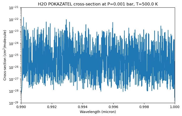
The cross-sections are stored in a 3D array with the shape (n_pressures, n_temperatures, n_wavenumbers). Here, we only have one pressure and temperature point, so we can just extract the first slice of the array. After that, we can plot the cross-sections.
[18]:
fig, ax = plt.subplots(figsize=(8, 5))
ax.plot(1/wavenumbers * 1e4, cross_section_slice[0, 0, :])  # convert wavenumber to wavelength in micron
ax.set_xlabel('Wavelength (micron)')
ax.set_ylabel('Cross-section (cm$^2$/molecule)')
ax.set_title(f'H2O POKAZATEL cross-section at P={pressures[0]} bar, T={temperatures[0]} K')
ax.set_yscale('log')
ax.set_xlim(0.99, 1.0)
ax.set_ylim(1e-29, 1e-21);
If you want to convert the file to the pRT format afterward, you can use the following function. For that you need to have a working petitRADTRANS installation. A guide on how to install petitRADTRANS can be found here.
If you use the pRT format, please provide the DOI of the line list you used for the calculation, so that it is stored in the file. Additionally, you can provide information you want to include into the file. The standard information includes the isotope list, the line racer version, the line list name, the broadening species dictionary, the broadening type, the cutoff and which sub-Lorentzian corrections were used.
The rewrite parameter controls whether to overwrite an already existing file with the same name. If you want to keep the old file if one exists, set it to False. Additionally, if you want to use the petitRADTRANS input file path for storing the converted file, set use_prt_input_file_path=True. Note, that if you choose that and rewrite=True, your current pRT opacities are overwritten. If set to False, the files are stored in the prt format, but in a folder in the current
working directory called cross-sections_prt_format/. It will automatically calculate the opacities in the standard correlated-k and line-by-line format of petitRADTRANS.
[19]:
add_info = "this was a test calculation of H2O opacities using line racer."
doi = "10.1093/mnras/sty1877"  # doi of the line list

H2O_racer.convert_opacity_to_prt_format(final_cross_section_file_name, doi, rewrite=True, additional_information=add_info, use_prt_input_file_path=False)
Generating petitRADTRANS wavenumber grid... Done.
Reading opacity files in directory '.temporary_pRT_xsec_1H2-16O_POKAZATEL'...
Starting conversion of directory '.temporary_pRT_xsec_1H2-16O_POKAZATEL'...
 Reading file '.temporary_pRT_xsec_1H2-16O_POKAZATEL/xsec_1H2-16O_1.00e-03bar_500K.zarr' (1/1)... Done.
Preparation successful
Starting line-by-line conversion (boundaries: [ 0.3 28. ])...
Creating directory '/Users/haegele/codes/line_racer/docs/content/notebooks/cross-sections_prt_format/opacities/lines/line_by_line/H2O/1H2-16O'
 Writing line-by-line file '/Users/haegele/codes/line_racer/docs/content/notebooks/cross-sections_prt_format/opacities/lines/line_by_line/H2O/1H2-16O/1H2-16O__POKAZATEL.R1e6_0.3-28mu.xsec.petitRADTRANS.h5'...
Successfully converted files in '.temporary_pRT_xsec_1H2-16O_POKAZATEL' to line-by-line pRT files
Starting correlated-k conversion (R = 1000)...
 Reshaping...
 Initializing correlated-k parameters...
 Calculating correlated-k (20/7728)...
/Users/haegele/codes/line_racer/.pixi/envs/default/lib/python3.11/site-packages/petitRADTRANS/__file_conversion.py:3139: UserWarning: directory '.temporary_pRT_xsec_1H2-16O_POKAZATEL' contains only 1 files, the standard petitRADTRANS temperature-pressure grid size is 130; a finer temperature-pressure grid allows for a more accurate interpolation of the cross-sections
  warnings.warn(f"directory '{opacities_directory}' contains only {len(opacity_files)} files, "
 Done.lating correlated-k (7728/7728)...
Creating directory '/Users/haegele/codes/line_racer/docs/content/notebooks/cross-sections_prt_format/opacities/lines/correlated_k/H2O/1H2-16O'
 Writing file '/Users/haegele/codes/line_racer/docs/content/notebooks/cross-sections_prt_format/opacities/lines/correlated_k/H2O/1H2-16O/1H2-16O__POKAZATEL.R1000_0.1-250mu.ktable.petitRADTRANS.h5'...
Successfully converted files in '.temporary_pRT_xsec_1H2-16O_POKAZATEL' to correlated-k pRT files
Removed temporary folder .temporary_pRT_xsec_1H2-16O_POKAZATEL with the individual p T point files.
We can ignore the warning about the number of files, since we only used one pressure temperature point for demonstration purposes. In practice, you would use the whole line list or at least all files covering the wavelength region of interest. The resulting file can be directly used in petitRADTRANS.
Using HITRAN line lists#
A guide on how to download HITRAN line lists can be found in the downloading line list data tutorial. To download HITRAN data, you need to be logged in on the HITRAN website. Therefore, we will download the demonstration data from a cloud, just to show how the calculation works. If you want to use the HITRAN data for real, please download the line list files from the HITRAN website.
We will calculate the HITRAN CO2 line list here. Credit for the data goes to these papers. First we need to set up the folder structure.
[20]:
os.makedirs('line_list/CO2', exist_ok=True)
After that, we are downloading the line list data. As mentioned, it is downloaded from a cloud using urllib.request. If that is not working for you, please download it manually from HITRAN or here. However, the partition function can be downloaded from the HITRAN website directly. For HITRAN data the .par file is needed, which contains all line information, especially the broadening for air and self. If you want to use more
or other broadening species, please have a look at the downloading line list data tutorial. Additionally, the partition function data is needed, which is stored in a .txt file.
[21]:
urllib.request.urlretrieve('https://keeper.mpdl.mpg.de/f/3b4ddd913b7e44e984fe/?dl=1', 'line_list/CO2/69300f3e.par')
urllib.request.urlretrieve("https://hitran.org/data/Q/q7.txt", "line_list/CO2/q7.txt")
[21]:
('line_list/CO2/q7.txt', <http.client.HTTPMessage at 0x302846950>)
As for ExoMol, we need to define the pressure and temperature grid. Here, we are only using one pressure and temperature point for demonstration purposes. If you want to use a pre-defined petitRADTRANS grid, you can use the function lr.LineRacer.prt_pressure_temperature_grid() as shown in the ExoMol example.
[22]:
pressures = [1.0]  # in bar
temperatures = [1500.0]  # in K
After that, we can define the line racer object, which already contains most of the relevant information for our opacity calculation. In general, everything is written in lower case letters, except for the line list name, since it is only used for naming the output files.
[23]:
CO2_racer = lr.LineRacer(resolution=1e6,
                         cutoff=100.0,  # in 1/cm
                         lambda_min=1.1e-5,  # in cm
                         lambda_max=2.5e-2,  # in cm
                         grid_type='log',
                         sublorentzian="Hartmann",
                         database='hitran',
                         input_folder='line_list/CO2/',  # path to folder with input files
                         temperatures=temperatures,  # in K
                         pressures=pressures,  # in bar
                         species_isotope_dict={'12C-16O2': 1.0},  # dictionary with the name of the isotope(s) in ExoMol convention and their number fraction(s)
                         line_list_name='HITRAN2024',
                         broadening_species_dict={'air': 1.0},
                         broadening_type='hitran_table',  # could also be 'sharp_burrows', 'hitran_table' or 'constant'

                         # Change the following only if you know what you do!
                         force_molliere2015_below_wn=40,  # use the Mollière et al. 2015 method for lines with effective wavenumbers smaller than this threshold.
                         force_molliere2015_method=False  # whether to force using Mollière et al. (2015) for line profile calculation, recommended only if warning appears or for small line lists
                         )
A detailed description of the class constructor can be found in the ExoMol section. Here, we will just explain the differences.
The input folder where the line list files (.par/.out, .txt) are stored is now the one containing the HITRAN files, the naming convention of the dictionary with the isotopes to calculate is still in the ExoMol naming convention and will be translated internally. Since the HITRAN line lists do not have specific names, we just call it ‘HITRAN2024’. For the dictionary with the broadening species air and self are possible for .par files, since their information is included there.
For self-created .out files the species names as seen on the HITRAN website in the output format description are required as an input here. As a broadening type, the ‘hitran_table’ is used, which stands for the broadening parameters included in the .par or .out file. The molecular mass is not required for HITRAN line lists, since it is read from the molparam.txt file automatically.
The explanation for force_molliere2015_methodand force_molliere2015_below_wn can be found in the ExoMol section.
HITRAN intensities are weighted by their natural abundance by default. In line racer, this is automatically corrected for and the opacities are scaled to abundance 1. If you want a different abundance, such as the natural abundance, you can set the desired abundance in the species_isotope_dict.
We also need to prepare the calculation by setting up the wavelength grid. Finally, we can provide the transition files list directly here, or let line racer search for all .par or .out files in the input folder. If there are .par and .out files, the .out files are preferred.
[24]:
transition_files_list = CO2_racer.prepare_opacity_calculation()
print("The transition file(s) to be used for the calculation are: ", transition_files_list)
The transition file(s) to be used for the calculation are: ['line_list/CO2/69300f3e.par']
After preparing the calculation, we can start the actual opacity calculation. Here, we can also choose whether to use MPI for parallelization or not. If you are on a cluster and have MPI set up, you can set use_mpi=True to use it. Otherwise, just set it to False and line racer will use multiprocessing for parallelization. In the case of normal multiprocessing (use_mpi=False) you can choose the number of cores by setting n_cores to
the number of cores you want to use.
If you are using the line_racer_obj.calculate_opacity in a script make sure to put it in a if __name__ == "__main__": block to avoid problems with multiprocessing.
You can either directly use the petitRADTRANS format by setting prt_format=True or first calculate the cross-sections in line racer’s own format, which is a zarr compressed with zip. More about that, and which further information are needed for the petitRADTRANS format can be found in the ExoMol section. Here, they are set to None. We use the flag verbose=True, to get more information about the line calculation.
For calculations with HITRAN line lists additionally to the intensity correction files, the molparam.txt file is needed, which is downloaded automatically if not present in the data/ folder. More about the intensity correction can be found in the ExoMol section and the intensity correction chapter.
[25]:
final_cross_section_file_name = CO2_racer.calculate_opacity(transition_files_list,
                                                            use_mpi=False,
                                                            n_cores=1,
                                                            sampling_boost=1.0,
                                                            coarse_grid_switch=True,

                                                            # pRT output options
                                                            prt_format=False,
                                                            doi=None,
                                                            additional_information=None,
                                                            use_prt_input_file_path=False,

                                                            # more output
                                                            verbose=True)

print("The cross-sections are stored in the file: ", final_cross_section_file_name)
Using cutoff and Hartmann intensity correction grid and interpolated to 100.0 1/cm
Reading HITRAN transition file...
Finished reading HITRAN transition file in 1.09 seconds.


 Line parameter calculation time: 0.013465166091918945 s
Starting the line profile calculation of 174446 lines

 Starting internal lines!
Line profile calculation done
 Internal lines done!
 Starting external lines!
Progress: 770/773 subgrids
 External lines done!
Total time for opacity calculation:  41.73415803909302 s

The cross-sections are stored in the file:  cross-sections/cross-section_12C-16O2__HITRAN2024__40-90909cm-1.zarr.zip
The resulting cross-section file is stored in the folder cross-sections/ by default. The file contains the pressure grid in bar and temperature grid in Kelvin, the wavenumber grid in 1/cm and the cross-sections in \(\rm cm^2/molecule\) for each pressure and temperature point. If you want to convert the cross-sections to the petitRADTRANS format, you could directly set prt_format=True in the calculate_opacity function or just convert it afterward, as explained in the ExoMol
section.
[26]:
store = zarr.storage.ZipStore(final_cross_section_file_name, mode='a')
z = zarr.group(store=store)

# Access datasets
pressures = z['pressures'][:]
temperatures = z['temperatures'][:]
wavenumbers = z['wavenumbers'][:]
cross_section = z['cross-sections']

print("Pressures (bar): ", pressures)
print("Temperatures (K): ", temperatures)

# Extract slice and plot
cross_section_slice = cross_section[:]
Pressures (bar):  [1.]
Temperatures (K):  [1500.]
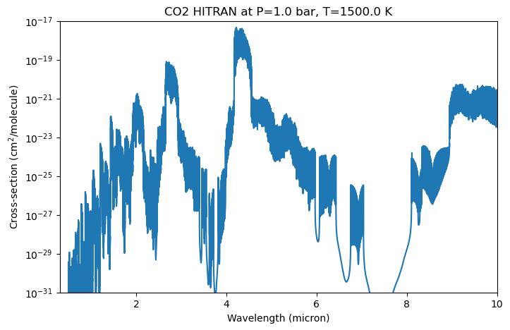
[27]:
fig, ax = plt.subplots(figsize=(8, 5))
ax.plot(1/wavenumbers * 1e4, cross_section_slice[0, 0, :])  # convert wavenumber to wavelength in micron

ax.set_xlabel('Wavelength (micron)')
ax.set_ylabel('Cross-section (cm$^2$/molecule)')
ax.set_title(f'CO2 HITRAN at P={pressures[0]} bar, T={temperatures[0]} K')
ax.set_yscale('log')
ax.set_ylim(1e-31, 1e-17)
ax.set_xlim(0.3, 10);
Using HITEMP line lists#
A guide on how to download HITEMP line lists can be found in the downloading line list data tutorial. To download HITEMP data, you need to be logged in on the HITRAN website. Therefore, we will download the demonstration data from a cloud, just to show how the calculation works. If you want to use the HITEMP data for real, please download the line list files from the HITRAN website.
We will calculate the HITEMP CO line list here. Credit for the data goes to G. Li et al. 2015. First we need to set up the folder structure.
[28]:
os.makedirs('line_list/CO', exist_ok=True)
After that, we are downloading the line list data. As mentioned, it is downloaded from a cloud using urllib.request. If that is not working for you, please download it manually from HITRAN or here. However, the partition function can be downloaded from the HITRAN website directly. For HITRAN data the .par file is needed, which contains all line information. Additionally, the partition function data is needed, which is stored in a
.txt file.
[29]:
urllib.request.urlretrieve('https://keeper.mpdl.mpg.de/f/be281779a65542db814e/?dl=1', 'line_list/CO/05_HITEMP2019.par')
urllib.request.urlretrieve('https://hitran.org/data/Q/q26.txt', 'line_list/CO/q26.txt')
[29]:
('line_list/CO/q26.txt', <http.client.HTTPMessage at 0x32c0697d0>)
As for ExoMol, we need to define the pressure and temperature grid. Here, we are only using one pressure and temperature point for demonstration purposes. If you want to use a pre-defined petitRADTRANS grid, you can use the function lr.LineRacer.prt_pressure_temperature_grid() as shown in the ExoMol example.
[30]:
pressures = [1.0]  # in bar
temperatures = [1500.0]  # in K
After that, we can define the line racer object, which already contains most of the relevant information for our opacity calculation. In general, everything is written in lower case letters, except for the line list name, since it is only used for naming the output files.
[31]:
CO_racer = lr.LineRacer(resolution=1e6,
                         cutoff=100.0,  # in 1/cm
                         lambda_min=1.1e-5,  # in cm
                         lambda_max=2.5e-2,  # in cm
                         grid_type='log',
                         sublorentzian="Hartmann",
                         database='hitemp',
                         input_folder='line_list/CO/',  # path to folder with input files
                         temperatures=temperatures,  # in K
                         pressures=pressures,  # in bar
                         species_isotope_dict={'12C-16O': 1.0},
                         line_list_name='HITEMP2019',  # you can specify the version here
                         broadening_species_dict={'air': 1.0},
                         broadening_type='hitran_table',  # could also be 'sharp_burrows', 'hitran_table' or 'constant'

                         # Change the following only if you know what you do!
                         force_molliere2015_below_wn=40,  # use the Mollière et al. 2015 method for lines with effective wavenumbers smaller than this threshold.
                         force_molliere2015_method=False  # whether to force using Mollière et al. (2015) for line profile calculation, recommended only if warning appears or for small line lists
                         )
A detailed description of the class can be found in the ExoMol section. Here, we will just explain the differences.
The input folder where the line list files (.par/.out, .txt) are stored is now the one containing the HITEMP files. The naming convention of the dictionary with the isotopes to calculate is still in the ExoMol naming convention and will be translated internally. Since the HITEMP line lists do not have specific names, we just call it ‘HITEMP2019’. For the dictionary with the broadening species air and self is possible for .par files. The broadening species is air and the
broadening type HITRAN table, since HITRAN is the provider of the HITEMP line lists. The molecular mass is not required for HITEMP line lists, since it is read from the molparam.txt file automatically.
The explanation for force_molliere2015_methodand force_molliere2015_below_wn can be found in the ExoMol section.
HITEMP intensities are weighted by their natural abundance by default. In line racer, this is automatically corrected for and the opacities are scaled to abundance 1. If you want a different abundance, such as the natural abundance, you can set the desired abundance in the species_isotope_dict.
We also need to prepare the calculation by setting up the wavelength grid. Finally, we can provide the transition files list directly here, or let line racer search for all .par files in the input folder.
[32]:
transition_files_list = CO_racer.prepare_opacity_calculation()

print("The transition file(s) to be used for the calculation are: ", transition_files_list)
The transition file(s) to be used for the calculation are: ['line_list/CO/05_HITEMP2019.par']
After preparing the calculation, we can start the actual opacity calculation. Here, we can also choose whether to use MPI for parallelization or not. If you are on a cluster and have MPI set up, you can set use_mpi=True to use it. Otherwise, just set it to False and line racer will use multiprocessing for parallelization. In the case of normal multiprocessing (use_mpi=False) you can choose the number of cores by setting n_cores to
the number of cores you want to use.
If you are using the line_racer_obj.calculate_opacity in a script make sure to put it in a if __name__ == "__main__": block to avoid problems with multiprocessing.
You can either directly use the petitRADTRANS format by setting prt_format=True or first calculate the cross-sections in line racer’s own format, which is a zarr compressed with zip. More about that, and which further information are needed for the petitRADTRANS format can be found in the ExoMol section. Here, they are set to None. We use the flag verbose=True, to get more information about the line calculation. In addition to the intensity correction files, HITEMP
calculations also need the molparam.txt file, which is downloaded automatically if not present in the data/ folder.
[33]:
# calculate the final cross-sections
final_cross_section_file_name = CO_racer.calculate_opacity(transition_files_list,
                                                           use_mpi=False,
                                                           n_cores=1,
                                                           sampling_boost=1.0,
                                                           coarse_grid_switch=True,

                                                           # pRT output options
                                                           prt_format=False,
                                                           doi=None,
                                                           additional_information=None,
                                                           use_prt_input_file_path=False,

                                                           # more output
                                                           verbose=True)

print("The cross-sections are stored in the file: ", final_cross_section_file_name)
Using cutoff and Hartmann intensity correction grid and interpolated to 100.0 1/cm
Reading HITRAN transition file...
Finished reading HITRAN transition file in 3.48 seconds.


 Line parameter calculation time: 0.011228084564208984 s
Starting the line profile calculation of 125496 lines

 Starting internal lines!
Line profile calculation done
 Internal lines done!
 Starting external lines!
Progress: 770/773 subgrids
 External lines done!
Total time for opacity calculation:  51.39884614944458 s

The cross-sections are stored in the file:  cross-sections/cross-section_12C-16O__HITEMP2019__40-90909cm-1.zarr.zip
The resulting cross-section file is stored in the folder cross-sections/ by default. The file contains the pressure grid in bar and temperature grid in Kelvin, the wavenumber grid in 1/cm and the cross-sections in \(\rm cm^2/molecule\) for each pressure and temperature point. If you want to convert the cross-sections to the petitRADTRANS format, you could directly set prt_format=True in the calculate_opacity function or just convert it afterward, as explained in the ExoMol
section.
[34]:
store = zarr.storage.ZipStore(final_cross_section_file_name, mode='a')
z = zarr.group(store=store)

# Access datasets
pressures = z['pressures'][:]
temperatures = z['temperatures'][:]
wavenumbers = z['wavenumbers'][:]
cross_section = z['cross-sections']

print("Pressures (bar): ", pressures)
print("Temperatures (K): ", temperatures)

# Extract slice and plot
cross_section_slice = cross_section[:]
Pressures (bar):  [1.]
Temperatures (K):  [1500.]
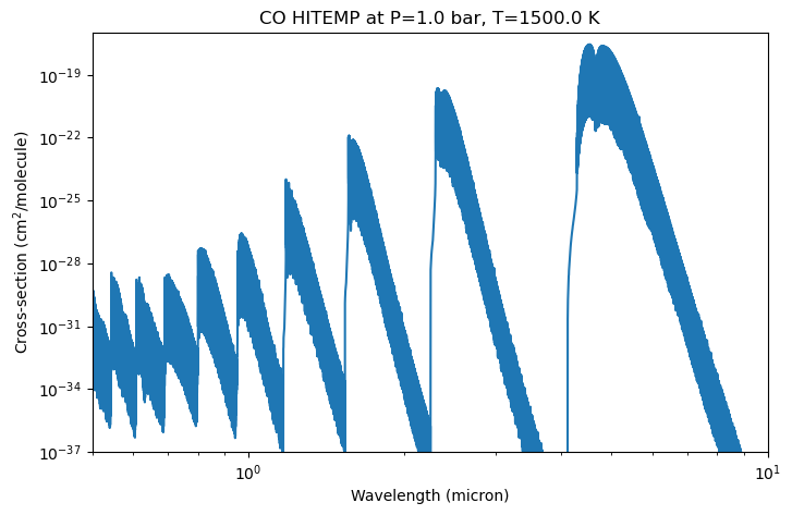
[35]:
fig, ax = plt.subplots(figsize=(8, 5))
ax.plot(1/wavenumbers * 1e4, cross_section_slice[0, 0, :])  # convert wavenumber to wavelength in micron

ax.set_xlabel('Wavelength (micron)')
ax.set_ylabel('Cross-section (cm$^2$/molecule)')
ax.set_title(f'CO HITEMP at P={pressures[0]} bar, T={temperatures[0]} K')
ax.set_yscale('log')
ax.set_xscale('log')
ax.set_ylim(1e-37, 1e-17)
ax.set_xlim(0.5, 10);
Intensity Correction#
Because of the cutoff or sub-Lorentzian treatment of the line wings, the total line intensity is not conserved anymore. To account for that, line racer uses pre-calculated intensity correction grids. These are downloaded by default when you prepare the opacity calculation for the first time. However, if that does not work, you can download them manually from this link and store the files in a folder data/. The pre-calculated grid
ranges from Gaussian widths of \(10^{-6}\) to 100 1/cm, gamma/sigma ratios from \(10^{-9}\) to \(10^{6}\) and cutoff values from 1 to 5000 1/cm. The grid has 500 points in the width direction and 100 points in the gamma/sigma ratio and cutoff direction. The intensity correction is calculated for three cases: with Hartmann et al. (2002) corrections, Burch et al. (1969) corrections, and cutoff only. Depending on whether you use the Hartmann or Burch corrections or not, the respective
grid is used for the intensity correction. If your cutoff is larger than 5000 1/cm, no intensity correction is applied. If the line widths are outside the range of the correction grid, the nearest value is used.
You can also calculate the grids manually by running the following code, for example if you want to use a larger cutoff or range of line widths. The grids are stored in the data/ folder. More about the intensity correction and how it works can be found in the background information of the line calculation.
[36]:
from line_racer.intensity_correction_precalculation import calculate_correction_grid

# Define parameters for the correction grid calculation
gamma_sigma_ratio_minimum = 1e-9
gamma_sigma_ratio_maximum = 1e6
sigma_minimum = 1e-6
sigma_maximum = 1e2
width_points = 50  # normally 500!!!
cutoff_minimum = 1
cutoff_maximum = 5000
cutoff_points = 1  # normally 100!!!

os.makedirs("dataa/", exist_ok=True)

# calculate the grid for the Hartmann and cutoff correction
Hartmann = True
hartmann_cutoff_correction_grid, sigma_grid, gamma_sigma_ratio_grid, cutoff_grid = calculate_correction_grid(
                                                                            gamma_sigma_ratio_minimum,
                                                                            gamma_sigma_ratio_maximum,
                                                                            sigma_minimum, sigma_maximum, width_points,
                                                                            cutoff_minimum, cutoff_maximum,
                                                                            cutoff_points, use_hartmann=Hartmann)
np.savez('dataa/correction_grid_hartmann_cutoff.npz', sigma_grid=sigma_grid, gamma_sigma_ratio_grid=gamma_sigma_ratio_grid,
         cutoff_grid=cutoff_grid, correction_grid=hartmann_cutoff_correction_grid)

# calculate the grid for the Hartmann and cutoff correction
Burch = True
burch_cutoff_correction_grid, sigma_grid, gamma_sigma_ratio_grid, cutoff_grid = calculate_correction_grid(
                                                                            gamma_sigma_ratio_minimum,
                                                                            gamma_sigma_ratio_maximum,
                                                                            sigma_minimum, sigma_maximum, width_points,
                                                                            cutoff_minimum, cutoff_maximum,
                                                                            cutoff_points, use_burch=Burch)
np.savez('dataa/correction_grid_burch_cutoff.npz', sigma_grid=sigma_grid, gamma_sigma_ratio_grid=gamma_sigma_ratio_grid,
         cutoff_grid=cutoff_grid, correction_grid=burch_cutoff_correction_grid)

# calculate the grid for the cutoff correction only
cutoff_correction_grid, sigma_grid, gamma_sigma_ratio_grid, cutoff_grid = calculate_correction_grid(
                                                                            gamma_sigma_ratio_minimum,
                                                                            gamma_sigma_ratio_maximum,
                                                                            sigma_minimum, sigma_maximum, width_points,
                                                                            cutoff_minimum, cutoff_maximum,
                                                                            cutoff_points)
np.savez('dataa/correction_grid_cutoff.npz', sigma_grid=sigma_grid, gamma_sigma_ratio_grid=gamma_sigma_ratio_grid,
         cutoff_grid=cutoff_grid, correction_grid=cutoff_correction_grid)

import shutil
shutil.rmtree("dataa/")
Calculating correction grid for cutoff and using Hartmann correction 1.00 cm^-1 (1/1)
Calculating correction grid for cutoff 1.00 cm^-1 (1/1)
For calculation time reasons, we are just using one cutoff value and 50 width values here for the grid and also create a folder dataa/ instead of data/. In practice, you would want to use 100 cutoff points and store the files in the data/ folder.
Splitting up huge ExoMol .trans files#
Some of the ExoMol .trans files are very large (up to 100 GB), which can cause problems with memory and make multiprocessing inefficient or impossible. Therefore, line racer provides a function to split up the huge .trans files into smaller files, which directly store the important line parameters in a .npz file. With that, only these smaller files have to be read in for the opacity calculation, which is much faster and more efficient. The splitting up is recommended if you want to
calculate opacities from line lists that contain many lines but are not split up into smaller files. Examples are the ExoMol line lists for H2CS, which contain 43 billion lines in just eight files. But also for the ExoMol MM line list for CH4 it is recommended to split up the files, since some of the files are over 35GB in size, which makes multiprocessing on one node
very difficult for typical node memory. With the split files, the multiprocessing automatically uses the smaller files and the calculation is much faster and more efficient. It is recommended to use this function, if you ran into memory problems or if you want to optimize the multiprocessing and therefore the speed of the calculation.
For demonstration purposes, we will split up one file from the ExoMol MM line list for CH4. First we need to download the .trans file(s) we want to split up and the .states file, which contains the energy levels and is needed for the splitting up. The smaller files later directly store the important line parameters, such as the effective wavenumber, the Einstein A coefficient, the lower energy level, the upper state degeneracy and the upper and lower state rotational quantum number. The
splitting up is done in bins of a certain width, which can be set as an input. The smaller files are stored in the same folder as the original .trans file. The original .trans file is not deleted, so you can always go back to it if needed. However, they could be deleted after the splitting up if you want to save disk space, since they are not needed anymore for the opacity calculation. The smaller files are named with the original file name and the bin wavenumbers, so that they can be
easily identified and used for the opacity calculation.
[37]:
os.makedirs('line_list/CH4', exist_ok=True)

base = "https://www.exomol.com/db/CH4/12C-1H4/MM"

files = {
    f"{base}/12C-1H4__MM.states.bz2" : "line_list/CH4/12C-1H4__MM.states.bz2",
    f"{base}/12C-1H4__MM__01000-01100.trans.bz2" : "line_list/CH4/12C-1H4__MM__01000-01100.trans.bz2"
}

for url, dest in files.items():
    if not os.path.exists(dest):
        urllib.request.urlretrieve(url, dest)
In this case we use the compressed .bz2 files, which slows down the process, but is easier for demonstration purposes. It also works with the uncompressed files at two times the speed, since the reading in of the files is faster.
[38]:
pressures, temperatures = lr.LineRacer.prt_pressure_temperature_grid()

CH4_racer = lr.LineRacer(database='exomol',
                         mass=16.03130013,
                         input_folder='line_list/CH4/',  # path to folder with input files
                         temperatures=temperatures,  # in K
                         pressures=pressures,  # in bar
                         species_isotope_dict={'12C-1H4': 1.0},
                         line_list_name='MM',
                         broadening_type='exomol_table',
                         broadening_species_dict={'H2': 0.85, 'He': 0.15},
                         )

CH4_racer.split_huge_transition_files(transition_files_list=None, bin_width=10.0, use_mpi=True)
Splitting line_list/CH4/12C-1H4__MM__01000-01100.trans.bz2 took 78.00282406806946 seconds
For the line racer object here, only the relevant information for the splitting up is needed, such as the input folder and the line list name. The pressures, temperatures and broadening information are not relevant for the splitting up, but are required when constructing the object. For the splitting up, you can either provide the transition files list directly or let line racer search for all .trans files in the input folder. The bin_width parameter controls the width of the bins in
which the lines are split up. The smaller the bin width, the smaller the resulting files, but also the more files are created. A good value for the bin width depends on the line density of the line list, on the size of the original files and the available memory. For very large files and high line density, a smaller bin width is recommended to make sure that the resulting files are not too large. The splitting up is parallelized with MPI, so you can set use_mpi=True if you have MPI set up on
your cluster.